Clustering projects according to similarities in outcomes they achieve

Among some users of LogFrames it is verboten to have more than one Purpose level (i.e. outcome) statement. They are likely to argue that where there are multiple intended outcomes a project's efforts will be dissipated and will ultimately be ineffective. However, a reasonable counter-argument would be that in some cases multiple outcome measures may simply be more nuanced description of an outcome that others might want to insist is expressed in a singular form.

The "problem" of multiple outcome measures becomes more common when we look at portfolios of projects where there may be one or two over-arching objectives but it is recognised that there are multiple pathways to their achievement. Or, that it is recognized that individual projects may want to trying different mixes of strategies , rather than just one alone.

How can an evaluator deal with multiple outcomes, and data on these? Some years ago one strategy that I used was to gather the project staff together to identify for each output, what its expected relative causal contribution was of each of the project outcomes. These judgements were expressed in individual values that added up to 100 percentage points per outcome, plotted in an (Excel) Outputs x Outcome matrix, projected onto a screen for all to see, argue and edit. The results enabled us to prioritise which Output to Outcome linkages to give further attention to, and to identify, in aggregate, which Outputs would need more attention than others.

There is also another possible approach. More recently I have been exploring the potential uses of clustering modules within the RapidMiner data mining package. I have a data set of 34 projects with data on their achievements on 11 different outcome measures. A month ago I was contracted to develop some predictive models for each of these outcomes, which I did. But it now occurs to me that doing so may be somewhat redundant, in that there may not really be 11 different types of project performance. Rather, it is possible that there are a smaller number of clusters of projects, and within each of these there are projects having similar patterns of achievement across the various possible outcomes.

With this in mind I have been exploring the use of two different clustering algorithms: (k-Means clustering and DBSCAN clustering. Both are described in practically useful detail in Kotu and Deshpande's book "Predictive Analytics and Data Mining"

With k-Means you have to specify the number of clusters you are looking for (k), which may be useful in some circumstances. but I would prefer to find an "ideal" number. This could be the number of clusters where there is the highest level of similarity of cases within a cluster compared to other alternative numbers of clusterings of the same cases. The performance metrics of k-Means clustering allows this kind of assessment to be made. The best performing clustering result I found identified four clusters. With DBSCAN you don't nominate any preferred number of clusters, but it turns out there are other parameters you do need to set, which also affect the result, including the number of clusters found. But again, you can compare and assess these using a performance measure, which I did. However, in this case the best performing result was two clusters rather than four!

What to do? Talk to the owners of the data, who know the details of the cases involved and show them the alternative clustering, including information on which projects belong to which clusters. Then ask them which clustering makes the most sense i.e. is most interpretable, given their knowledge of these projects.

And then what? Having identified the preferred clustering model it would make sense then to go back to the full data set and develop predictive models for these clusters: i.e. to find what package of project attributes will best predict the particular cluster of outcome achievements that are of interest.

Evolving better performing hypotheses, using Excel

You may not know this, but there is an Excel add-in called Solver. This can be used to evolve better solutions to computation problems.

It can also be used to identify hypotheses that have a better fit with available data. Here is how I have been using Solver in Excel....

I start by entering a data set into Excel that is made up of cases (e.g.25 projects), listed row by row. The columns then describe attributes of those projects, e.g. as captured in project completion reports. These attributes can include aspects of the project context, the way the project was working plus some outcome performance measures.

A filtering mechanism is then set up in Excel, where you can chose a specific sub-set of the attributes that are of interest (aka our hypothesis), and then all the projects that have these attributes are automatically highlighted.

The performance of this sub-set of projects is then tested, using a simple device called a Confusion Matrix , which tells us what proportion of the selected projects have "successful" versus "unsuccessful" outcomes (if that is the outcome of interest). Ideally, if we have selected the right set of attributes then the proportion of "successful" projects in the selected sub-set will be greater than their prevalence rate in the whole set of projects.

But given that the number of possible hypotheses available to test doubles with each extra attribute added into the data set, this sort of intuitive/theory led search could take us a long time to find the best available solution. Especially when the data set has a large number of attributes.

This is where Solver helps. Using its evolutionary algorithm the Solver add-in provides a quick means of searching a very large space of possible solutions. To do this there are three parameter which need to be set, before setting it to work. The first is the Objective, which is the value you want to maximise. I usually choose the "Accuracy" measure in the Confusion Matrix. The second is the range of cells whose values can be varied. These are the ones identifying the set of project attributes, which can be used to make a hypothesis. They can be set to (1), absent (0) or not relevant (2). The third is is the Constraints, which limit the values that these variable cells can take e.g. not negative, and nothing other than these three types of values.

In the space of a minute Solver then explores up to 70,000 possible combinations of project attributes to find the combination that generate the most accurate prediction i.e. a set of projects with the highest possible proportion of "successful" projects. In my recent trials, using a real data set, the accuracy levels have been up around 90%. I have been able to compare the results with those found using another algorithm which I have written about in earlier posts here, called a  Decision Tree algorithm. Despite being quite different algorithms, the solutions that both algorithms have found (i.e. the specific set of project attributes) have been very similar in content (i.e. the attributes in the solution), and both had the same level of accuracy.

An important side benefit of this approach to finding out "what works" is that by manually tweaking the solutions found by Solver you can measure the extent to which each attribute in the winning solution makes a difference to its overall accuracy. This is the kind of question many donors want to answer re the projects they fund, when they ask "What difference does my particular contribution make?"

If you want help setting up Excel to try out this method, and have a data set ready to work on, feel free to contact me for advice: rick.davies@gmail.com, or leave a comment below

Is QCA it's own worst enemy?

[As you may have read elsewhere on this blog] QCA stands for Qualitative Comparative Analysis. It is a method that is finding increased use as an evaluation tool, especially for exploring claims about the causal role of interventions of various kinds. What I like about it is its ability to recognize and analyse complex causal configurations, which have some fit with the complexity of the real world as we know it.

What I don't like about it is its complexity, it can sometimes be annoyingly obscure and excessively complicated. This is a serious problem if you want to see the method being used more widely and if you want the results to be effectively communicated and properly understood. I have seen instances recently where this has been such a problem that it threatened to derail an ongoing evaluation.

In this blog post I want to highlight where the QCA methodology is unnecessary complex and and suggest some ways to avoid this type of problem. In fact I will start with the simple solution, then explain how QCA manages to make it more complex.

Let me start with a relatively simple perspective. QCA analyses fall in to the broad category of "classifiers". These include a variety of algorithmic processes for deciding what category various instances belongs to. For example which types of projects were successful or not in achieving their objectives.

I will start with a two by two table, a Truth Table, showing the various possible results that can be found, by QCA and other methods. Configuration X here is a particular combination of conditions that an analysis has found to be associated with the presence of an outcome. The Truth Table helps us identify just how good that association is, by comparing the incidences where the configuration is present or absent with the incidences where the outcome is present or absent.

As I have explained in an earlier blog, one way of assessing the adequately of the result shown in such a matrix is by using a statistical test such as Chi Square, to see if the distribution is significantly different from what a chance distribution would look like.There are only two possible results when the outcome is present: the association is statistically significant or it is not.

However, if you import the ideas of Necessary and/or Sufficient causes the range of interesting results increases. The matrix can now show four possible types of results when the outcome is present:

1. The configuration of conditions is Necessary and Sufficient for the outcome to be present. Here cells C and B would be empty of cases
2. The configuration of conditions is Necessary but Insufficient for the outcome to be present. Here cell C would be empty of cases
3. The configuration of conditions is Unnecessary but Sufficient for the outcome to be present. Here cell  B would be empty of cases
4. The configuration of conditions is Unnecessary and Insufficient for the outcome to be present. Here no cells would be empty of cases

The interesting thing about the first three options is that they are easy to disprove. There only needs to be one case found in the cell(s) meant to be empty, for that claim to be falsified.

And we can provide a lot more nuance to the type 4 results, by looking at the proportion of cases found in cells B and C, relative to cell A. The proportion of A/(A+B) tells us about the consistency of the results, in the simple sense of consistency of results found via an examination of a QCA Truth Table. The proportion of A/(A+B) tells us about the coverage of the results, as in the proportion of all present outcomes that exist that were identified by the configuration. 

So how does QCA deal with all this? Well, as far as I can see, it does so in a way makes it more complex than necessary. Here I am basing my understanding mainly on Schneider and Wagemann's account of QCA.

1. Firstly, they leave aside the simplest notions of Necessity and Sufficiency as described above, which are based on a categorical notion of Necessity and Sufficiency i..e a configuration either is or is not Sufficient etc. One of the arguments I have seen for doing this is these types of results are rare and part of this may be due to measurement error, so we should take  more generous/less demanding view of what constitutes Necessity and Sufficiency
2. Instead they focus on Truth Tables with results as shown below (classed as 4. Unnecessary and Insufficient above). They then propose ways of analyzing these in terms of having degrees of Necessity and Sufficiency conditions. This involves two counter-intuitive mirror-opposite ways of measuring the consistency and coverage of the results, according to whether the focus is on analyzing the extent of Sufficiency or Necessity conditions (see Chapter 5 for details)
3. Further complicating the analysis is the introduction of a minimum thresholds for the consistency of Necessity and Sufficiency conditions (because the more basic categorical idea has been put aside). There is no straightforward basis for defining these levels. It is suggested that they depend on the nature of the problem being identified.

  Configuration X contains conditions which are neither Necessary or Sufficient 

Using my strict interpretation of Sufficiency and Necessity there is no need for a consistency measure where a condition (or configuration) is found to be Sufficient but Unnecessary, because there will be no cases in cell B. Likewise, there is no need for a coverage measure where a condition (or configuration) is found to be Necessary but Insufficient, because there will be no cells in cell C,

We do need to know the consistency where a condition (or configuration) is Necessary but Insufficient, and the the coverage, where where a condition (or configuration) is found to be Sufficient but Unnecessary.

Characterising purposive samples

In some situations it is not possible to develop a random sample of cases to examine for evaluation purposes. There may be more immediate challenges, such as finding enough cases with sufficient information and sufficient quality of information.

The problem then is knowing to what extent, if at all, the findings from this purposive sample can be generalised, even in the more informal sense of speculating on the relevance of findings to other cases in the same general population.

One way this process can be facilitated is by "characterising" the sample, a term I have taken from elsewhere. It means to describe the distinctive features of something. This could best be done using attributes or measures that can, and probably already have been, used to describe the wider population where the sample came from. For example, the sample of people could be described as being of average age of 35 versus 25 in the whole population, and 35% women versus 55% in the wider population. This seems a rather basic idea, but it is not always applied.

Another more holistic way of doing so is to measure the diversity of the sample. This is relatively easy to do when the data set associated with the sample is in binary form, as for example is used in QCA analysis (i.e. cases are rows, columns are attributes and cell values of 0 or 1 indicate if the attributes was absent or present)

As noted in earlier blog postings,Simpsons Reciprocal Index is a useful measure of diversity. This takes into account two aspects of diversity: (a) richness, which in a data set could be seen in the number of unique configurations of attributes found across all the cases( think metaphorically of organisms - cases, chromosomes-configurations and genes-attributes) and (b) evenness, which could be seen in the relative number of cases having particular configurations. When the number of cases is evenly distributed across all configurations this is seen as being more diverse than when the number of cases per configuration varies.

The degree of diversity in a data base can have consequences. Where a data set that has little diversity in terms of "richness" there is a possibility that configurations that are identified by QCA or other algorithmic based methods, will have limited external validity, because they may easily be contradicted by cases outside the sample data set that are different from already encountered configurations. A simple way of measuring this form of diversity is to calculate the original number of unique configurations in the sample data set as a percentage of the total number possible, given the number of binary attributes in the sample data set (which is 2 to the power of the number of attributes). The higher the percentage, the less risk that the findings will be contradicted by configurations found in new sets of data (all other things being constant).

Where a data set has little diversity in terms of "balance" it will be more difficult to assess the consistency of any configuration's association with an outcome, compared to others, because there will be more cases associated with some configurations than others. Where there are more cases of a given configuration there will be more opportunities for its consistency of association with an outcome to be challenged by contrary cases.

My suggestion therefore is that when results are published from the analysis of purposive samples there should be adequate characterisation of the sample, both in terms of: (a) simple descriptive statistics available on the sample and wider population, and (b) the internal diversity of the sample, relative to the maximum scores possible on the two aspects of diversity.

Evaluating the performance of binary predictions

(Updated 2015 06 06)

Background: This blog posting has its origins in a recent review of a QCA oriented evaluation, in which a number of hypotheses were proposed and then tested using a QCA type data set. In these data set cases (projects) are listed row by row and the attributes of these projects are listed in columns. Additional columns to the right describe associated outcomes of interest. The attributes of the projects may include features of the context as well as the interventions involved. The cell values in the data sets were binary (1=attribute present, 0= not present), though there are other options.

When such a data set is available a search can be made for configurations of conditions that are strongly associated with an outcome of interest. This can be done inductively or deductively. Inductive searches involve the uses of systematic search processes (aka algorithms), of which there are a number available. QCA uses the Quine–McCluskey algorithm. Deductive searches involve the development of specific hypotheses from a body of theory, for example about the relationship between the context, intervention and outcome.

Regardless of which approach is used, the resulting claims of association need evaluation. There are a number of different approaches to doing this that I know of, and probably more. All involve, in the simplest form, the analysis of a truth table in this form:

In this truth table the cell values refer to the number of cases that have each combination of configuration and outcome. For further reference below I will label each cell as A and B (top row) and C and D (bottom row)

The first approach to testing is a statistical approach. I am sure that there are a number of ways of doing this, but the one I am most familiar with is the widely used Chi-Square test. Results will be seen as most statistically significant when all cases  are in the A and D cells. They will be least significant when they are equally distributed across all four cells.

The second approach to testing is the one used by QCA. There are two performance measures. One is Consistency, which is the proportion of all cases where the configuration is present and the outcome is also present (=A/(A+B)). The other is Coverage, which is the proportion of all outcomes that are associated with the configuration (=(A/(A+C)).

When some of the cells have 0 values three categorical judgements can also be made. If only cell B is empty then it can be said that the configuration is Sufficient but not Necessary. Because there are still values in cell C this means there are other ways of achieving the outcome in addition to this configuration.

If only cell C is empty then it can be said that the configuration is Necessary but not Sufficient. Because there are still values in cell B this means there are other additional conditions that are needed to ensure the outcome.

If cells B and C are empty then it can be said that the configuration is both Necessary and Sufficient

In all three situations there only needs to be one case to be found in a previously empty cell(s) to disprove the standing proposition. This is a logical test, not a statistical test.

The third approach is one used in the field of machine learning, where the above matrix is known as a Confusion Matrix. Here there is a profusion of performance measures available (at least 13). Some of the more immediately useful measures are:

• Accuracy: (A+D)/(A+B+C+D), which is similar to but different from the Chi Square measure above
• True Positives: A/(A+B), also called Precision, which corresponds to QCA consistency
• True Negatives: D/(B+D)
• False Positives: C/(A+C)
• False Negatives: B/(B+D)
• Positive predictive value: A/(A+C), also called Recall, which corresponds to QCA coverage
• Negative predictive value: D/(C+D)

In addition to these three types of tests there are three other criteria that are worth taking into account as well: simplicity, diversity and similarity

Simplicity: Essentially the same idea as that captured in Occam's Razor. This is that simpler configurations are preferable, all other things being equal. For example: A+F+J leads to D is a simpler hypothesis than A+X+Y+W+F leads to D. Complex configurations can have a better fit with the data, but at the cost of being poor at generalising to other contexts. In Decision Tree modelling this is called "over-fitting" and solution is "pruning", i.e. cutting back on the complexity of the configuration.  Simplicity has practical value, when it comes to applying tested hypotheses in real life programmes. They are easier to communicate and to implement. Simplicity can be measured at two levels: (a) the number of attributes in a configuration that is associated with an outcome, (b) and the number of configurations needed to account for an outcome.

Diversity: The diversity of configurations is simply the number of different specific configurations in a data set. It can be made into a comparable measure by calculating it as a percentage of the total number possible. The total number possible is 2 to the power of A where A = number of kinds of attributes in the data set. A bigger percentage = more diversity.

If you want to find how "robust" a hypothesis is, you could calculate the diversity present in the configurations of all the cases covered by the hypothesis (i.e. not just the attributes specified by the hypotheses, which will be all the same). If that percentage is large this suggests the hypothesis works in a greater diversity of circumstances, a feature that could be of real practical value.

This notion of diversity is to some extent implicit in the Coverage measure. More coverage implies more diversity of circumstances. But two hypotheses with the same coverage (i.e. proportion of cases they apply to) could be working in circumstances with quite different degrees of diversity (i.e. the cases covered were much more diverse in their overall configurations).

Similarity: Each row in a QCA like data set is a string of binary values. The similarity of these configurations of attributes can be measured in a number of ways:

• Jaccard index, the proportion of all instances in two configurations where the binary value 1 is present in the same position i.e. the same attribute is present.
• Hamming distance, the number of positions at which the corresponding values in two configurations are different. This includes the values 0 and 1, whereas Jaccard only looks at 1 values

These measures are relevant in two ways, which are discussed in more detail further down this post:

• If you want to find a "representative" case in a  data set, you would look for the case with the lowest average Hamming distance in the whole data set
• If you wanted to compare the two most similar cases, you would look for the pair of cases with the lowest Hamming distance.

Similarity can be seen as a third facet of diversity, a measure of the distance between any two types of cases. Stirling (2007) used the term disparity to describe the same thing.

Choosing relevant criteria: It is important to note that the relevance of these different association tests and criteria will depend on the context. A surgeon would want a very high level of consistency, even if it was at the cost of low coverage (i.e. applicable only in a limited range of situations). However, a stock market investor would be happy with a consistency of 0.55 (i.e 55%), especially if it had wide coverage. Even more so if that wide coverage contained a high level of diversity. Returning to the medical example, a false positive might have different consequences to false negatives e.g. unnecessary surgery versus unnecessary deaths. In other non-medical circumstances, false positives may be more expensive mistakes than false negatives.

Applying the criteria: My immediate interest is in the use of these kinds of tests for two evaluation purposes. The first is selective screening of hypotheses about causal configurations that are worth more time intensive investigations, an issue raised in a recent blog.

• Configurations that are Sufficient and not Necessary or Necessary but not Sufficient. 
• Among these, configurations which were Sufficient but not Necessary, and with high coverage should be selected, 
• And configurations which were Necessary but not Sufficient, and with high consistency, should also be selected. 
• Plus all configurations that were Sufficient and Necessary (which are likely to be less common)

The second purpose is to identify implications for more time consuming within-case investigations. These are essential, in order to identify casual mechanism at work that connect the conditions that are associated in a given configuration. As I have argued elsewhere, associations are a necessary but insufficient basis for a strong claim of causation. Evidence of mechanisms is like muscles on the bones of a body, enabling it to move.

Having done the filtering suggested above, the following kinds of within-case investigations would seem useful:

• Are there any common casual mechanisms underlying all the cases  found to be Necessary and Sufficient, i.e those within cell A? 
• A good starting point would be a case within this set of cases that had the lowest average Hamming distance, i.e. one with the highest level of similarity with all the other cases. 
• Once one or more plausible mechanism were discovered in that case a check could be made to see if they are present in other cases in that set, this could be done in two ways: (a) incrementally, by examining adjacent cases, i.e cases with the lowest Hamming distance from the representative case, (b) by partitioning the rest of the cases, and examining a case with a median level Hamming distance, i.e. half way between being the most similar and most different cases.
• Where the configuration is Necessary but not Sufficient, how do the cases in cell B differ from those in cell A, in ways that might shed more light on how the same configuration leads to different outcomes? This is what has been called a MostSimilarDifferentOutcome (MSDO) comparison,
• If there are many cases this could be quite a challenge, because the cases could differ on many dimensions (i.e. on many attributes). But using the Hamming distance measure we could make this problem more manageable by selecting a case from cell A and B that had the lowest possible Hamming distance. Then a within-case investigation could find additional undocumented differences that account for some or all of the difference in outcomes. 
• That difference could then be incorporated into the current hypothesis (and data set) enabling more cases from cell B to now be found in cell A i..e Consistency would be improved
• Where the configuration is Sufficient but not Necessary,in what ways are the cases in cell C the same as those in cell A, in ways that might shed more light on how the same outcome is achieved by different configurations? This is what has been called a MostDifferentSimilarOutcome (MDSO) comparison,
• As above, if there are many cases this could be quite a challenge. Here I am less clear, but de Meur et al (page 72) say the correct approach is "...one has to look for similarities in the characteristics of initiatives that differ the most from each other; firstly the identification of the most differing pair of cases and secondly the identification of similarities between those two cases" The within-case investigation should look for undocumented similarities that account for some of the similar outcomes. 
• That difference could then be incorporated into the current hypothesis (and data set) enabling more cases from cell C to now be found in cell A i..e Coverage would be improved

How to select which hypotheses to test?

I have been reviewing an evaluation that has made use of QCA (Qualitative Comparative Analysis). An important part of the report is the section on findings, which lists a number of hypotheses that have been tested and the results of those tests. All of these are fairly complex, involving a configuration of different contexts and interventions, as you might expect in a QCA oriented evaluation.  There were three main hypotheses, which in the results section were dis-aggregated into six more specific hypotheses. The question for me, which has  much wider relevance, is how do you select hypotheses for testing, given limited time and resources available in any evaluation?

The evaluation team have developed three different data sets, each will 11 cases, and with 6, 6 and 9 attributes of these cases (shown in columns), known as "conditions" in QCA jargon. This means there are 2⁶ + 2⁶  + 2⁹ = 640  possible combinations of these conditions that could be associated with and cause the outcome of interest. Each of the hypotheses being explored by the evaluation team represents one of these configurations. In this type of situation, the task of choosing an appropriate hypotheses seems a little like looking for a needle in a haystack

It seems there are at least three options, which could be combined. The first is to review the literature and find what claims (supported by evidence) are made there about "what works" and select from these those that are worth testing e.g. one that seems to have wide practical use, and/or one that could have different and significant program design implications if it is right or wrong. This seems to be the approach that the evaluation team has taken, though I am not so sure to what extent they have used the programming implications as an associated filter.

The second approach is to look for constituencies of interest among the staff of the client who has contracted the evaluation.There have been consultations, but it is not clear what sort of constituencies each of the tested hypotheses have. There were some early intimations that some of the hypotheses that were selected are not very understandable. That is clearly an important issue, potentially limiting the usage of the evaluation findings.

The third approach is an inductive search, using QCA or other software, for configurations of conditions associated with an outcome that have both high level of consistency (i.e. they are always associated with the presence (or the absence ) of an outcome) and  coverage (i.e. they apply to a large proportion of the outcomes of interest). In their barest form these configurations can be be considered as hypotheses. I was surprised to find that this approach had not been used, or at least reported on, in the evaluation report I read. If it had been used but no potentially useful configurations found then this should have been reported (as a fact, not a fault).

Somewhat incidentally, I have been playing around with the design of an Excel worksheet and managed to build in a set of formula for automatically testing how well different configurations of conditions of particular interest (aka hypotheses) account for a set of outcomes of interest, for a given data set. The tests involve measures taken from QCA (consistency and coverage, as above) and from machine learning practice (known as a Confusion Matrix). This set-up provides an opportunity to do some quick filtering of a larger number of hypotheses than an evaluation team might initially be willing to consider (i.e. the 6 above). It would not be as efficient a search as the QCA algorithm, but it would however be a search that could be directed according to specific interest. Ideally this directed search process would identify configurations that are both necessary and sufficient (for more than a small minority of outcomes). A second best result would be those that are necessary but insufficient, or vice versa. (I will elaborate on these possibilities and their measurement in another blog posting)

The wider point to make here is that with the availability of a quick screening capacity the evaluation team, in its consultations with the client, should then be able to broaden the focus of useful discussions away from what are currently quite specific hypotheses,  and towards the contents of a menu of a limited number of conditions that can not only make up these hypotheses but also other alternative versions. It is the choice of these particular conditions that will really make the difference, to the scale and usability of the results of a QCA oriented evaluation. More optimistically, the search facility could even be made available online, for continued use by those interested in the evaluation results, and their possible variants

The Excel file for quick hypotheses testing is here: http://wp.me/afibj-1ux

In defense of the (careful) use of algorithms and the need for dialogue between tacit (expertise) and explicit (rules) forms of knowledge

This blog posting is a response to the following paper now available online

Greenhalgh, T., Howick, J., Maskrey, N., 2014. Evidence based medicine: a movement in crisis? BMJ 348, http://www.bmj.com/content/348/bmj.g3725

Background: Chris Roche passed this very interesting paper on to me, received via "Kate", who posted a comment on  Chris's posting on "What has cancer taught me about the links between medicine and development? which can be found on Duncan Green's "From Poverty to Power" blog. 

The paper is interesting in the first instance because both the debate and practice about evidence based policy and practice seems to be much further ahead in the field of medicine than it is in the field of development aid (...broad generalisation that this is...).

It is also of interest to reflect on the problems and solutions copied below and to think how many of these kinds of issues can also be seen in development aid programs.

 According to the paper, the problems with the current version of evidence based medicine include:

1. Distortion of the evidence based brand ("The first problem is that the evidence based “quality mark” has been misappropriated and distorted by vested interests. In particular, the drug and medical devices industries increasingly set the research agenda. They define what counts as disease ... They also decide which tests and treatments will  be compared in empirical studies and choose (often surrogate) outcome measures for establishing “efficacy.”
2. Too much evidence:  The second aspect of evidence based medicine’s crisis (and yet, ironically, also a measure of its success) is the sheer volume of evidence available. In particular, the number of clinical guidelines is now both unmanageable and unfathomable. One 2005 audit of a 24 hour medical take in an acute hospital, for example, included 18 patients with 44 diagnoses and identified 3679 pages of national guidelines (an estimated 122 hours ofreading) relevant to their immediate care"
3. Marginal gains and a shift from disease to risk: "Large trials designed to achieve marginal gains in a near saturated therapeutic field typically overestimate potential benefits (because trial samples are unrepresentative and, if the trial is overpowered, effects may be statistically but not clinically significant) and underestimate harms (because adverse events tend to be under detected or under reported)."
4. Overemphasis on following algorithmic rules: "Well intentioned efforts to automate use of evidence through computerised decision support systems, structured templates, and point of care prompts can crowd out the local,individualised, and patient initiated elements of the clinical consultation"
5. Poor fit for multi-morbidity. "Multi-morbidity (a single condition only in name) affects every person differently and seems to defy efforts to produce or apply objective scores, metrics, interventions, or guidelines"

The paper's proposed solutions or ways forward include:

1. Individualised for the patient: Real evidence based medicine has the care of individual patients as its top priority, asking, “what is the best course of action for this patient, in these circumstances, at this point in their illness or condition?” It consciously and reflexively refuses to let process (doing tests, prescribing medicines) dominate outcomes (the agreed goal of management in an individual case). 
2. Judgment not rules. Real evidence based medicine is not bound by rules.  
3. Aligned with professional, relationship based care.  Research evidence may still be key to making the right decision—but it does not determine that decision. Clinicians may provide information, but they are also trained to make ethical and technical judgments, and they hold a socially recognised role to care, comfort, and bear witness to suffering.
4. Public health dimension . Although we have focused on individual clinical care, there is also an important evidence base relating to population level interventions aimed at improving public health (such as pricing and labelling of consumables, fluoridation of water, and sex education). These are often complex, multifaceted programmes with important ethical and practical dimensions, but the same principles apply as in clinical care. 
5. Delivering real evidence based medicine. To deliver real evidence based medicine, the movement’s stakeholders must be proactive and persistent. Patients (for whose care the movement exists) must demand better evidence, better presented, better explained, and applied in a more personalised way with sensitivity to context and individual goals.
6. Training must be reoriented from rule following Critical appraisal skills—including basic numeracy, electronic database searching, and the ability systematically to ask questions of a research study—are prerequisites for competence in evidence based medicine. But clinicians need to be able to apply them to real case examples.
7. Evidence must be usable as well as robust. Another precondition for real evidence based medicine is that those who produce and summarise research evidence must attend more closely to the needs of those who might use it
8. Publishers must raise the bar. This raises an imperative for publishing standards. Just as journal editors shifted the expression of probability from potentially misleading P values to more meaningful confidence intervals by requiring them in publication standards, so they should now raise the bar for authors to improve the usability of evidence, and especially to require that research findings are presented in a way that informs individualised conversations.
9. ...and more

While many of these complaints and claims that make a lot of sense, I think there is also a risk"throwing the baby out with the bathwater" if care is not taken with some. I will focus on a couple of ideas that run through the paper.

The risk lies in seeing two alternative modes of practice as exclusive choices. One is rule based, focused on average affects when trying to meet common needs in populations and the other is expertise focused on the specific and often unique needs of individuals. Parallels could be drawn between different type of aid programs, e.g. centrally planned and nationally rolled out services meeting basic needs like water supply or education and much more person centered participatory rural development programs

Alternatively, one can see these two approaches as having complementary roles that can help and enrich each other. The authors describe one theory of learning which probably applies in many fields, including medicine: The first stage " ...beginning with the novice who learns the basic rules and applies them mechanically with no attention to context. The next two stages involve increasing depth of knowledge and sensitivity to context when applying rules. In the fourth and fifth stages, rule following gives way to expert judgments, characterised by rapid, intuitive reasoning informed by imagination, common sense, and judiciously selected research evidence and other rules"  During this process a lot of explicit knowledge become tacit, and almost automated, with conscious attention left for the more case specific features of a situation. It is an economic use of human cognitive powers. Michael Polanyi wrote about this process years ago (1966, The Tacit Dimension).

The other side of this process is when tacit knowledge gets converted into explicit knowledge. That's what some anthropologists and ethnographers do. They seek to get into the inner world of their subjects and to make it accessible to others. One practitioner whose work interests me in particular is Christina Gladwin, who wrote a book on Ethnographic Decision Trees in 1989. This was all about eliciting how people, like small farmers in west Africa, made decisions about what crops to plant. The result was a decision tree model, that summarised all the key choices farmers could make, and the final outcomes those different choices would lead to. This was not  a model of how they actually thought, but a model of how different combinations of choices were associated with different outcomes of interest. These decision trees are not so far removed from those used in medical practice today.

A new farmer coming into the same location could arguably make use of such a decision tree to decide what to crops to plant. Alternatively they could work with one of the farmers for a number of seasons, which then might cover all the eventualities in the decision tree, and learn from that direct experience. But this would take much more time. In this type of setting explicit rule based knowledge is an  easier and quicker means of transferring knowledge between people. Rule based knowledge that can be quickly and reliably communicated is also testable knowledge.  Following the same pattern of rules may or may not always lead to the expected outcome in another context.

And now a word about algorithms. An algorithm is a clearly defined sequence of steps that will lead to a desired end, sometimes involving some iteration until that end state gets closer. A sequence of choices in a decision tree is an algorithm. At each choice point the answer will dictate what choices to be made next. These are the rules mentioned in the paper above. There are also algorithms for constructing such algorithms. On this blog I have made a number of postings about QCA and (automated) Decision Tree models, both of which are means of constructing testable causal models. Both involve computerised processes for finding rules that best predict outcomes of interest. I think they have a lot of potential in the field of development aid.

But returning to the problems of evidence based medicine, it is very important to note that algorithms are means of achieving specific goals. Deciding which goals need to be pursued remains a very human choice. Even within the use of both QCA and (automated) Decision tree modeling users have to decide the extent to which they want to focus on finding rules that are very accurate or those which are less accurate but which apply to a wider range of circumstances (usually simple rather than complex rules).

So, in summary, in any move towards evidence based practice, we need to ensure that tacit and explicit forms of knowledge build upon each other rather than getting separated as different and competing forms of knowledge. And while we should develop, test and use good algorithms, we should remember they are always means to an end, and we remain responsible for choosing the ends we are trying to achieve.

Postscript 2015 05 04: Please also read this recent cautionary analysis of the use of algorithms for the purposes of public policy implementation. The author points out that algorithms can embody and perpetuate cultural biases. How is that possible? It is possible because all evidence-based algorithms are developed using historical data i.e. data sets of what has happened in the past. Those data sets, e.g. of arrest and conviction data in a given city reflect historical practice by human institutions in that city, with all their biases, conscious and not so conscious. They don't reflect ideal practice, simply the actual practice at the time. Where an algorithm is not based on analysis of historical data then it may have its origins in a more ethnographic study of the practice of human experts in the domain of interest. Their practice, and their interpretations of their practice, are also equally subject to cultural biases. The analysis by Virginia Eubanks include four useful suggestions to counter these risks, one of which is that "We need to learn more about how policy algorithms work" by demanding more transparency about the design of a given algorithm and its decisions. But this may not be possible, or in some cases publicly desirable. One alternative method of interest is the algorithmic audit.

A mistaken criticism of the value of binary data

When reviewing a recent evaluation report I came across the following comment:

"Crisp set QCA where binary codings are used to establish the presence or absence of certain conditions does not facilitate a nuanced or granular analysis."

(PS: Look here for the basics of QCA) 

Wrong. Simply wrong.

A DFID strategy for promoting "improved governance" could be coded  as present or absent. This does seem crude, given the varieties of ways in which a governance strategy could actually be implemented. But the answer is not to ditch binary coding, but to extend it.

This can be done by breaking down the concept of "a strategy for improved governance"  into a number of component parts or attributes, and then coding for their presence/absence. The initial conception of the governance strategy is then deemed present if all 10 attributes are present. But it only takes a single change in one attribute at a time to produce 9 new versions of almost the same strategy. If you change two attributes at a time, there are ( 1 think... 1-(10 x 10) =) 100 new versions. If any number of attributes can be changed then this means there are 2 to the power of 10 possible configurations of the strategy, some of which may be very different from the present strategy. Basically it does not take much tweaking of the initial configuration before you will have nuances by the bucketful!

The limitations of the dis-aggregation-into-components approach have nothing to do with the nature of binary coding, but rather whether there are enough cases available to allow identification of the kinds of outcomes associated with the different varieties of configurations arising from the more micro-level coding of attributes.

If there are enough cases available, then learning about what works through the emergence (or planned development) of variations in the initial configuration then becomes possible. Some of these new versions of a governance strategy may work more effectively than the initial model, and others less so. Incremental exploration becomes possible.

For more on the idea of exploring adjacent variations in causal configurations see Andreas Wagner's very interesting (2014) book titled "The Arrival of the Fittest" which explores a theory of how innovation is possible in biological systems. Here is a review of the book, in the Times Higher Education website.

There is also a connection here, I think, with Stuart Kauffman's concept of "the adjacent possible", an idea also taken up by Stephen Johnson in his book "Where do good ideas come from: The natural history of innovation" Here is a review of the book in the Guardian

Postscript 2015 05 14: I heard the same"binary is crude"  criticism again today from a person attending a QCA presentation at the UK Evaluation Society Conference in London.

This time I will present another response. Binary judgments can be and often are derived from a dichotomised scale that captures graduations of the phenomena of interest. As Carroll Patterson pointed out today, with current QCA software it is now possible to experiment with varying the location of the cut-off point on such scales, and observe the consequences for the quality of the configurations that are then identified as the best fitting solutions The same approach is also possible with searches for best-fitting configurations using an evolutionary algorithm, which is another approach I have been experimenting with recently. It is also possible to go much further into the specific details of the underlying concept being measured by a scale by basing it on the aggregated output of a weighted checklist, like the kind I have described elsewhere. Basically, the limit to what is possible is defined by the imagination of the researcher/evaluator, not any inherent limitation of binary measures.

Postscript  2015 05 17: I tried to post a Comment below in reply to Anon's comment below, but Blogger.com wont accept any HTML formatting, so I will place the comment here instead.

RE "If, to combat the reductiveness of binary coding, you introduce a scale of 4-6 points, you still face the same problem in coding something more complex – a remote non expert is reducing a complex context and process to a number in an arbitrary way. "

Coding for QCA (and other purposes, such as when using NVIVO) should always be done in a way that is transparent and replicable, with attention to inter-rate reliability. It should certainly not be done in an “arbitrary way”

RE "Grading a large, diverse and complicated country on a scale of 0-1 or 1-5 on 'improved governance' is just ridiculous. Anyone who has studied the way people actually behave, governance, how decisions are really made or projects succeed or fail, will tell you that this reductiveness does not helpfully or accurately reflect reality."

QCA has been used in a field of Political Science since the 1980s and many of these applications have been cross-country analyses of political systems.

RE QCA is not qualitative – as it seeks to reduce a complex qualitative issue to a quantitative score - a number.

In crisp-set QCA data set the “number” 0 or 1 is actually a category not a numerical value. QCA could be done just as well by replacing  the 0’s and 1’s with the words “absent” and “present” 

RE "QCA is not comparative – the serious comparative part comes afterwards in some form of qualitative analysis, which researchers can choose. Looking at the truth table for patterns is the only form of comparison that QCA offers."

There are two levels of analysis involved in QCA: within-case analysis and between-case analysis.  At the beginning within-case analysis informs the selection of conditions to be included in a data set. When inconsistencies are found in an examination of configurations in a data set good practice advises a return to within-case analysis to identify missing conditions that can resolve these inconsistencies.  When these have been resolved and set of configurations has been identified that accounts for all case in the most parsimonious way possible,  these then need to be interpreted by reference to   the details of specific cases, with particular attention to more detailed process that connect the conditions making up the configurations.

RE "In my view QCA is a quantitative form of data management and pattern identification."

It does depend on what you mean by quantitative. It is based on a form of mathematics known as set theory, but that is about logical relationships, not quantities. In case there is any reservation about its significance, pattern identification is very important. In a data set with 10 different conditions there are 2 to the 10 different possible combinations of these that might be consistently associated with an outcome of interest. Finding these is like looking for a needle in a haystack. QCA and other methods like decision tree algorithms, help us find what part of the haystack the needle is most likely to be found. But as I said at the end of my section of the UKES presentation, finding a plausible configuration is not enough. It is necessary but not sufficient  for a strong causal claim. There also needs to be a plausible account of the likely causal mechanisms at work that connect the conditions in the configurations. These will only be found and confirmed through detailed within-case investigations, using methods like (but not only) process tracing. And the pattern finding has to be systematic, and transparent in the way it has been done. This is the case with QCA and Decision Tree modeling, where there are specifics algorithms used, both with their known limitations

There is a useful reference that may be of interest: Wagemann, C., Schneider, C.Q., 2007. Standards of Good Practice in Qualitative Comparative Analysis (qca) and Fuzzy-Sets. http://www.compasss.org/wpseries/WagemannSchneider2007.pdf

Comparing QCA and Decision Tree models - an ongoing discussion

This blog is a continuation of a dialogue that is based on Michaela Raab and Wolfgang Stuppert's  EVAW blog. I would have preferred to post my response below via their blog's Comment facility, but it cant cope with long responses or hypertext links. They in turn have had difficulty posting comments on my YouTube site where this EES presentation (Triangulating the results of Qualitative Comparative Analyses (EES Dublin 2014)  can be seen. It was this presentation that prompted their response here on their blog.

Hi Michaela and Wolfgang

Thanks for going to the trouble of responding in detail to my EES presentation.

Before responding in detail I should point out to readers that the EES presentation was on the subject of triangulation, and how to compare QCA and Decision Tree models, when applied to the same data set. In my own view I think it is unlikely that either of these methods will produce the “best” results in all circumstances. The interesting challenge is to develop ways of thinking about how to compare and choose between specific models generated by these, and what may be other comparable methods of analysis. The penultimate slide (#17)  in the presentation highlights the options I think we can try out when faced with different kinds of differences between models.

The rest of this post responds to particular points that have been made by Michaela and Wolfgang, and then makes a more general conclusion.

Re  “1. The  decision tree analysis is not based on the same data set as our QCA” This is correct. I was in a bit of a quandary because while the original data set was fuzzy set (i.e. there intermediate values between 0 and 1) the solutions that were found were described in binary form i.e. the conditions and outcomes either were or were not present. I did produce a Decision Tree with the fuzzy set data but I had no easy means of comparing the results with the binary results of the QCA model. That said, Michaela and Wolfgang are right in expecting that such a model would be more complex and have more configurations.

Re “2. Decision tree analysis is compared with a type of QCA solution that is not meant to maximise parsimony.”  I agree that “If the purpose was to compare the parsimony of QCA results with those of decision trees, then the 'parsimonious' QCA solution should be used” But the intermediate solution was the solution that was available to me, and parsimony was not the only criteria of interest in my presentation. Accuracy (or consistency in QCA terms) was also of interest. But it was the difference in parsimony that stood out the most in this particular model comparison.

Re “3. The decision tree analysis performs less well than stated in the presentation” Here I think I disagree. The focus of the presentation is on consistency of those configurations that predict effective evaluations only (indicated in the tree diagram by squares with 0.0 value rather than 1.0 value ), not the whole model.  Among the three configurations that predict effective evaluations the consistency was 82%. Slide 15 may have confused the discussion because the figures there refer to coverage rather than consistency (I should have made this clear).

Re “none of the paths in our QCA is redundant”. The basis for my claim here was some simple color coding of each case according to which QCA configuration applied to them. Looking back at the Excel file it appears to me that cases 14 and 16 were covered by two configurations and cases 16 and 32 by another two configurations. BUT bear in mind this was done with the binary (crisp) data, not the fuzzy valued data. (The two configurations that did not seem to cover unique cases were  quanqca*sensit*parti_2  and qualqca*quanqca*sensit*compevi_3). The important point here is not that redundancy is “bad” but where it is found it can prompt us to think about how to investigate such cases if and when they arise (including when two different models provide alternate configurations for the same cases).

4. “The decision tree consistency measure is less rigorous than in QCA”       I am not sure that this matters in the case of the comparison at hand but it may matter when other comparisons are made. I say this because on the measures given on slide 13 the QCA model actually seems to perform better than the Decision Tree model. BUT again, a possibly confounding factor is the use of crisp versus fuzzy values behind the two measures. There is nevertheless a positive message here though, which is to look carefully into how the consistency measures are calculated for any two models being compared. On a wider note, there is an extensive array of performance measures for Decision Tree (aka classification) models that can be summarised in a structure known as a Confusion Matrix. Here is a good summary of these: http://www.saedsayad.com/model_evaluation_c.htm

Moving on, I am pleased that Michaela and Wolfgang have taken this extra step: “Intrigued by the idea of 'triangulating' QCA results with decision tree analysis, we have converted our QCA dataset into a binary format (as Rick did, see point 1 above) and conducted a csQCA with that data”. Their results show that the QCA model does better in three of four comparisons (twice on consistency levels and once on number of configurations). However, we differ in how to measure the performance of the Decision Tree model. Their count of configurations seem to involve double counting (4+4 for both types of outcome), whereas I count 3 and 2, reflecting a total of the 5 that exist in the tree. On this basis I see the Decision Tree model doing better on parsimony for both types of outcome but the QCA model doing better on consistency for both types of outcomes.

What would be really interesting to explore,  now that we have two more comparable models, is how much overlap there was in the contents of the configurations found by the two analyses, and the actual contents of those configurations i.e. the specific conditions involved. That is what will probably be of most interest to the donor (DFID) who funded the EVAW work. The findings could have operational consequences.

In addition to exploring the concrete differences between models based on the same data I think one other area that will be interesting to explore is how often the best levels of parsimony and accuracy can be found in one model versus one being available at the cost of the other in any given model. I suspect QCA may privilege consistency whereas Decision Tree algorithms might not do so. But this may simply reflect variations in analysis settings given for a particular analysis. This question has some wider relevance, since some parties might want to prioritise accuracy whereas others might want to prioritise parsimony. For example, a stock market investor could do well with a model that has 55% accuracy, whereas a surgeon might need 98%. Others might want to optimise both.

And a final word of thanks is appropriate, to Michaela and Wolfgang for making their data set publicly available for others to analyse. This is all too rare an event, but hopefully one that will become more common in the future, encouraged by donors and modeled by examples such as theirs.

Where is no common outcome measure...

The previous posting on this topic has now been removed but is still available as pdf  It was removed because I thought the solution it was exploring was too complex and would not really work very well, if at all!

Following some useful discussions with Comic Relief staff I have worked out a much simpler process, which I will describe below

The problem:

1. How do you make summary descriptive statements about the overall performance of a portfolio of activities, if there is no quantitative measure that can be applied to all projects in the portfolio? This kind of problem is likely to be present in projects with complex social development objectives e.g. those relating to accountability, empowerment, governance, etc.
2. How to identify the causal factors contributing to an outcome that seems to be unmeasurable because of its complexity? There are methods that can manage causal complexity, such as QCA and Decision Tree modelling which i have discussed elsewhere on this blog, but each of these are only practicable when there is some form of consistent coding of the type of outcomes that have occurred. 

The suggested approach to the outcome measurement problem: A multi-dimensional measure (MDM) for a given project = (The scale of achievement of the project specific outcomes) X (a weighting for the relative importance of that package of outcomes associated with a given project)

Project specific outcomes: Both DFID and DFAT (ex-AusAID) use a relatively simple annotated rating scale to assess the likely or actual achievement of a project’s objectives. By themselves these ratings can’t be sensibly aggregated, because the contents of the outcomes being achieved may be quite different. But this type of score can be used as an input to a larger calculation.

Where these rating systems are not in place a project specific rating can be generated through one of more types of pair comparison process. See Postscript 1 below.

Weightings: There are many different ways of developing weightings, some of which I have explored elsewhere. These weight individual aspects of performance then summarize these for each entity having those aspects. For example, the Basic Necessities Survey weights the importance of individual items households may posses, then sums the weights of all the items a household has into an aggregate score.

There is an alternate approach using a variant of the Hierarchical Card Sorting (HCS) process. This identifies clusters of performance attributes, then ranks them. Entities such as projects will have an outcome score that reflects their particular cluster of performance attributes.

• First stage: Participants are asked to sort projects in the portfolio of interest into two piles, to  “what they see as the most significant difference in the outcomes being sought by the projects, in the light of the overall objective of the portfolio, as they see it”. 

As with normal use of HCS, the same question is then re-iterated with each newly created group of projects to generate sub-groups of projects and then further sub-sub-groups.

The process stops when participants can no longer identify any significant differences, or when there is only one project left in any sub-group.

In facilitating this process care needs to be taken to ensure that participants do not start to report differences in the intervention, as distinct from outcomes. These are relevant to a causal analysis, but not to measurement of outcomes , which is the focus here.

The results from this first stage will be a nested classification in the form of a tree with various branches, each representing one or more projects pursuing a particular set of outcomes, as described by the multiple distinctions made at each point in the branch.

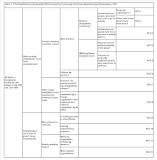
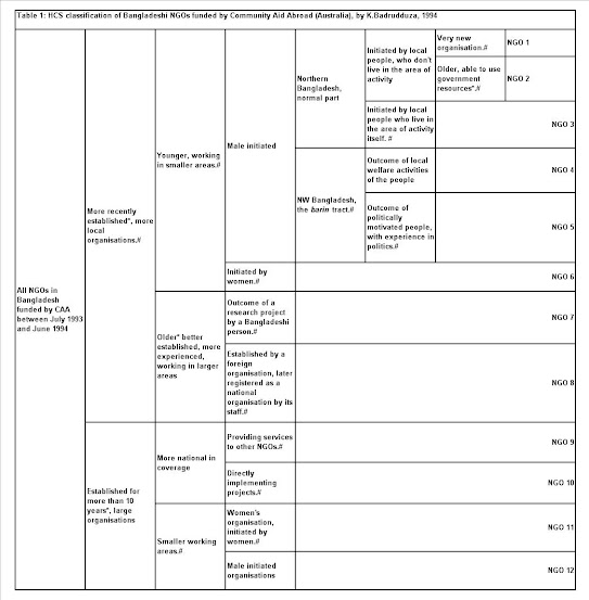
Here is an example of a hierarchical card sorting of projects funded in Bangladesh by an Australian NGO in the early 1990s [Caveat: It was developed way before the idea for this blog posting emerged, but it gives an idea of the type of tree structure that can be produced using a Hierarchical Card Sort. It is more focused on means rather than ends, so please bear this in mind.]

• Second stage: Participants are then asked to make choices at each branching point in the tree, starting from the base of the tree. They are asked to identify which type of outcome (represented by the two diverging branches) they think it is more important for the portfolio owner to be seeking to achieve. When this question is re-iterated down all branches of the tree this will enable a complete ranking of outcome configurations (branches) to be identified. 

Score construction: A simple table would then be generated in Excel where rows = projects and columns detailed (a) project specific ratings, (b) outcome weightings (i.e. the ranking of the branch that the project belonged to), (c) the product of the rating and weighting values.

Next: Now I need some real life examples, to show how this works in practice…and/or to discover the practical difficulties of using this approach. Any offers?


Postscript 1: Generating project ratings from pair comparisons. In my earlier version of this blog I explored the potential of a pair comparison method as a means of coming up with an overall ranking of project outcomes in a portfolio. The downside of this, as pointed out by Tom Thomas reflecting on PRA experiences, was that pair comparisons can be very time consuming and the time cost rises exponentially as the number of entities being compared increases.The number of pair comparaiosn = N to the power of N.

In the process of exploring this approach I ended up reading some of the literature on sorting algorithms. Processing cost (i.e. time taken to make comparisons of items) is one of the criteria that is used to assess the value of a sorting algorithm. Not surprisingly perhaps there is a huge variety of sorting algorithms. One which I have developed is described in this short Word file (NB: It was probably already developed by someone else many years ago!)

More recently still (April 2015), I have just finished reading Computational Fairy Tales by Jeremy Kubica, which I recommend to beginners in this area (such as me). In that book the author describes something called a QuickSort sorting algorithm, which sounds very useful for minimising the number of pair comparison needed to generate a complete ranking of a set of cases of interest. On average it works well, but in the worst case it can require N to the power of No comparisons. But this worst case wont apply when humans are doing the sorting because they can pick what are called "pivot" cases more purposively, whereas the computerised algorithm uses random choices. Good human choices of pivot cases with approximate median values should mean the sorting process is as quick as it can be with this type of algorithm.