Tuesday, October 07, 2014

Comparing QCA and Decision Tree models - an ongoing discussion


This blog is a continuation of a dialogue that is based on Michaela Raab and Wolfgang Stuppert's  EVAW blog. I would have preferred to post my response below via their blog's Comment facility, but it cant cope with long responses or hypertext links. They in turn have had difficulty posting comments on my YouTube site where this EES presentation (Triangulating the results of Qualitative Comparative Analyses (EES Dublin 2014)  can be seen. It was this presentation that prompted their response here on their blog.

Hi Michaela and Wolfgang

Thanks for going to the trouble of responding in detail to my EES presentation.

Before responding in detail I should point out to readers that the EES presentation was on the subject of triangulation, and how to compare QCA and Decision Tree models, when applied to the same data set. In my own view I think it is unlikely that either of these methods will produce the “best” results in all circumstances. The interesting challenge is to develop ways of thinking about how to compare and choose between specific models generated by these, and what may be other comparable methods of analysis. The penultimate slide (#17)  in the presentation highlights the options I think we can try out when faced with different kinds of differences between models.

The rest of this post responds to particular points that have been made by Michaela and Wolfgang, and then makes a more general conclusion.

Re  “1. The  decision tree analysis is not based on the same data set as our QCA” This is correct. I was in a bit of a quandary because while the original data set was fuzzy set (i.e. there intermediate values between 0 and 1) the solutions that were found were described in binary form i.e. the conditions and outcomes either were or were not present. I did produce a Decision Tree with the fuzzy set data but I had no easy means of comparing the results with the binary results of the QCA model. That said, Michaela and Wolfgang are right in expecting that such a model would be more complex and have more configurations.

Re “2. Decision tree analysis is compared with a type of QCA solution that is not meant to maximise parsimony.”  I agree that “If the purpose was to compare the parsimony of QCA results with those of decision trees, then the 'parsimonious' QCA solution should be used” But the intermediate solution was the solution that was available to me, and parsimony was not the only criteria of interest in my presentation. Accuracy (or consistency in QCA terms) was also of interest. But it was the difference in parsimony that stood out the most in this particular model comparison.

Re “3. The decision tree analysis performs less well than stated in the presentation” Here I think I disagree. The focus of the presentation is on consistency of those configurations that predict effective evaluations only (indicated in the tree diagram by squares with 0.0 value rather than 1.0 value ), not the whole model.  Among the three configurations that predict effective evaluations the consistency was 82%. Slide 15 may have confused the discussion because the figures there refer to coverage rather than consistency (I should have made this clear).

Re “none of the paths in our QCA is redundant”. The basis for my claim here was some simple color coding of each case according to which QCA configuration applied to them. Looking back at the Excel file it appears to me that cases 14 and 16 were covered by two configurations and cases 16 and 32 by another two configurations. BUT bear in mind this was done with the binary (crisp) data, not the fuzzy valued data. (The two configurations that did not seem to cover unique cases were  quanqca*sensit*parti_2  and qualqca*quanqca*sensit*compevi_3). The important point here is not that redundancy is “bad” but where it is found it can prompt us to think about how to investigate such cases if and when they arise (including when two different models provide alternate configurations for the same cases).

4. “The decision tree consistency measure is less rigorous than in QCA”       I am not sure that this matters in the case of the comparison at hand but it may matter when other comparisons are made. I say this because on the measures given on slide 13 the QCA model actually seems to perform better than the Decision Tree model. BUT again, a possibly confounding factor is the use of crisp versus fuzzy values behind the two measures. There is nevertheless a positive message here though, which is to look carefully into how the consistency measures are calculated for any two models being compared. On a wider note, there is an extensive array of performance measures for Decision Tree (aka classification) models that can be summarised in a structure known as a Confusion Matrix. Here is a good summary of these: http://www.saedsayad.com/model_evaluation_c.htm

Moving on, I am pleased that Michaela and Wolfgang have taken this extra step: “Intrigued by the idea of 'triangulating' QCA results with decision tree analysis, we have converted our QCA dataset into a binary format (as Rick did, see point 1 above) and conducted a csQCA with that data”. Their results show that the QCA model does better in three of four comparisons (twice on consistency levels and once on number of configurations). However, we differ in how to measure the performance of the Decision Tree model. Their count of configurations seem to involve double counting (4+4 for both types of outcome), whereas I count 3 and 2, reflecting a total of the 5 that exist in the tree. On this basis I see the Decision Tree model doing better on parsimony for both types of outcome but the QCA model doing better on consistency for both types of outcomes.

What would be really interesting to explore,  now that we have two more comparable models, is how much overlap there was in the contents of the configurations found by the two analyses, and the actual contents of those configurations i.e. the specific conditions involved. That is what will probably be of most interest to the donor (DFID) who funded the EVAW work. The findings could have operational consequences.

In addition to exploring the concrete differences between models based on the same data I think one other area that will be interesting to explore is how often the best levels of parsimony and accuracy can be found in one model versus one being available at the cost of the other in any given model. I suspect QCA may privilege consistency whereas Decision Tree algorithms might not do so. But this may simply reflect variations in analysis settings given for a particular analysis. This question has some wider relevance, since some parties might want to prioritise accuracy whereas others might want to prioritise parsimony. For example, a stock market investor could do well with a model that has 55% accuracy, whereas a surgeon might need 98%. Others might want to optimise both.

And a final word of thanks is appropriate, to Michaela and Wolfgang for making their data set publicly available for others to analyse. This is all too rare an event, but hopefully one that will become more common in the future, encouraged by donors and modeled by examples such as theirs.

Wednesday, July 23, 2014

Where is no common outcome measure...


The previous posting on this topic has now been removed but is still available as pdf  It was removed because I thought the solution it was exploring was too complex and would not really work very well, if at all!

Following some useful discussions with Comic Relief staff I have worked out a much simpler process, which I will describe below

The problem:

  1. How do you make summary descriptive statements about the overall performance of a portfolio of activities, if there is no quantitative measure that can be applied to all projects in the portfolio? This kind of problem is likely to be present in projects with complex social development objectives e.g. those relating to accountability, empowerment, governance, etc.
  2. How to identify the causal factors contributing to an outcome that seems to be unmeasurable because of its complexity? There are methods that can manage causal complexity, such as QCA and Decision Tree modelling which i have discussed elsewhere on this blog, but each of these are only practicable when there is some form of consistent coding of the type of outcomes that have occurred. 

The suggested approach to the outcome measurement problem: A multi-dimensional measure (MDM) for a given project = (The scale of achievement of the project specific outcomes) X (a weighting for the relative importance of that package of outcomes associated with a given project)

Project specific outcomes: Both DFID and DFAT (ex-AusAID) use a relatively simple annotated rating scale to assess the likely or actual achievement of a project’s objectives. By themselves these ratings can’t be sensibly aggregated, because the contents of the outcomes being achieved may be quite different. But this type of score can be used as an input to a larger calculation.

Where these rating systems are not in place a project specific rating can be generated through one of more types of pair comparison process. See Postscript 1 below.

Weightings: There are many different ways of developing weightings, some of which I have explored elsewhere. These weight individual aspects of performance then summarize these for each entity having those aspects. For example, the Basic Necessities Survey weights the importance of individual items households may posses, then sums the weights of all the items a household has into an aggregate score.

There is an alternate approach using a variant of the Hierarchical Card Sorting (HCS) process. This identifies clusters of performance attributes, then ranks them. Entities such as projects will have an outcome score that reflects their particular cluster of performance attributes.
  • First stage: Participants are asked to sort projects in the portfolio of interest into two piles, to  “what they see as the most significant difference in the outcomes being sought by the projects, in the light of the overall objective of the portfolio, as they see it”. 
As with normal use of HCS, the same question is then re-iterated with each newly created group of projects to generate sub-groups of projects and then further sub-sub-groups.
The process stops when participants can no longer identify any significant differences, or when there is only one project left in any sub-group.
In facilitating this process care needs to be taken to ensure that participants do not start to report differences in the intervention, as distinct from outcomes. These are relevant to a causal analysis, but not to measurement of outcomes , which is the focus here.
The results from this first stage will be a nested classification in the form of a tree with various branches, each representing one or more projects pursuing a particular set of outcomes, as described by the multiple distinctions made at each point in the branch.
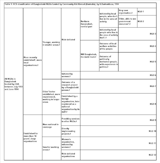
Here is an example of a hierarchical card sorting of projects funded in Bangladesh by an Australian NGO in the early 1990s [Caveat: It was developed way before the idea for this blog posting emerged, but it gives an idea of the type of tree structure that can be produced using a Hierarchical Card Sort. It is more focused on means rather than ends, so please bear this in mind.]


  • Second stage: Participants are then asked to make choices at each branching point in the tree, starting from the base of the tree. They are asked to identify which type of outcome (represented by the two diverging branches) they think it is more important for the portfolio owner to be seeking to achieve. When this question is re-iterated down all branches of the tree this will enable a complete ranking of outcome configurations (branches) to be identified. 

Score construction: A simple table would then be generated in Excel where rows = projects and columns detailed (a) project specific ratings, (b) outcome weightings (i.e. the ranking of the branch that the project belonged to), (c) the product of the rating and weighting values.

Next: Now I need some real life examples, to show how this works in practice…and/or to discover the practical difficulties of using this approach. Any offers?


Postscript 1: Generating project ratings from pair comparisons. In my earlier version of this blog I explored the potential of a pair comparison method as a means of coming up with an overall ranking of project outcomes in a portfolio. The downside of this, as pointed out by Tom Thomas reflecting on PRA experiences, was that pair comparisons can be very time consuming and the time cost rises exponentially as the number of entities being compared increases.The number of pair comparaiosn = N to the power of N.

In the process of exploring this approach I ended up reading some of the literature on sorting algorithms. Processing cost (i.e. time taken to make comparisons of items) is one of the criteria that is used to assess the value of a sorting algorithm. Not surprisingly perhaps there is a huge variety of sorting algorithms. One which I have developed is described in this short Word file (NB: It was probably already developed by someone else many years ago!)

More recently still (April 2015), I have just finished reading Computational Fairy Tales by Jeremy Kubica, which I recommend to beginners in this area (such as me). In that book the author describes something called a QuickSort sorting algorithm, which sounds very useful for minimising the number of pair comparison needed to generate a complete ranking of a set of cases of interest. On average it works well, but in the worst case it can require N to the power of No comparisons. But this worst case wont apply when humans are doing the sorting because they can pick what are called "pivot" cases more purposively, whereas the computerised algorithm uses random choices. Good human choices of pivot cases with approximate median values should mean the sorting process is as quick as it can be with this type of algorithm.


Friday, March 28, 2014

The challenges of using QCA


This blog posting is a response to my reading of the Inception Report written by the team who are undertaking a review of evaluations of interventions relating to violence against women and girls. The process of the review is well documented in a dedicated blog – EVAW Review

The Inception Report is well worth reading, which is not something I say about many evaluation reports! One reason is to benefit from the amount of careful attention the authors have given to the nuts and bolts of the process. Another is to see the kind of intensive questioning the process has been subjected to by the external quality assurance agents and the considered responses by the evaluation team. I found that many of the questions that came to my mind while reading the main text of the report were dealt with when I read the annex containing the issues raised by SEQUAS and the team’s responses to them.

I will focus on one issue that is challenge for both QCA and data mining methods like Decision Trees (which I have discussed elsewhere on this blog). That is the ratio of conditions to cases. In QCA conditions are attributes of the cases under examination that are provisionally considered as possible parts of causal configurations that explain at least some of the outcomes. After an exhaustive search and selection process the team has ended up with a set of 39 evaluations they will use as cases in a QCA analysis. After a close reading of these and other sources they have come up with a list of 20 conditions that might contribute to 5 different outcomes. With 20 different conditions there are 220 (i.e. 1,048,576) different possible configurations that could explain some or all of the outcomes. But there are only 39 evaluations, which at best will represent only 0.004% of the possible configurations. In QCA the remaining 1,048,537 are known as “logical remainders”. Some of these can usually be used in a QCA analysis through a process using explicit assumptions e.g. about particular configurations plus outcomes which by definition would be impossible to occur in real life. However, from what I understand of QCA practice, logical remainders would not usually exceed 50% of all possible configurations.

The review team has dealt with this problem by summarising the 20 conditions and 5 outcomes into 5 conditions and one outcome. This means there are 25 (i.e. 32) possible causal configurations, which is more reasonable considering there are 39 cases available to analyse. However there is a price to be paid for this solution, which is the increased level of abstraction/generality in the terms used to describe the conditions. This makes the task of coding the known cases more challenging and it will make the task of interpreting the results and then generalising from them more challenging as well. You can see the two versions of their model in the diagram below, taken from their report.
 
What fascinated me was the role of evaluation method in this model (see “Convincing methodology”). It is only one of five conditions that could explain some or all of the outcomes. It is quite possible therefore that all or some of the case outcomes could be explained without the use of this condition. This is quite radical, considering the centrality of evaluation methodology in much of the literature on evaluations. It may also be worrying to DFID in that one of their expectations of this review was it would “generate a robust understanding of the strengths, weaknesses and appropriateness of evaluation approaches and methods”. The other potential problem is that even if methodology is shown to be an important condition, its singular description does not provide any means to discriminating between forms which are more or less helpful.

The team seems to have responded to this problem by proposing additional QCA analyses, where there will be an additional condition that differentiates cases according to whether they used qualitative or quantitative methods.  However reviewers have still questioned whether this is sufficient. The team in return have commented that they will “add to the model further conditions that represent methodological choice after we have fully assessed the range of methodologies present in the set, to be able to differentiate between common methodological choices” It will be interesting to see how they go about doing this, while avoiding the problem of “insufficient diversity” of cases already mentioned above.

One possible way forward has been illustrated in a recent CIFOR Working Paper (Sehring et al, 2013) and which is also covered in Schneider and Wagemann (2012). They have illustrated how it is possible to do a “two-step QCA”, which differentiates between remote and proximate conditions. In the VAWG review this could take the form of an analysis of conditions other than methodology first, then a second analysis focusing on a number of methodology conditions. This process essentially reduces a larger number of remote conditions down to a smaller number of configurations that do make a difference to outcomes, which are then included in the second level of the analysis which uses the more proximate conditions. It has the effect of reducing the number of logical remainders. It will be interesting to see if this is the direction that the VAWG review team are heading.

PS 2014 03 30: I have found some further references to two-level QCA:
 And for people wanting a good introduction to QCA, see